Dynamic Water

Click anywhere to interact with objects or spawn crates. You can also change the quality of the water texture and reset the scene.

About

View this page without the runnable demo scene here.

The entire code of this project is hosted on GitHub. It is lincensed under MIT so feel free to do with it whatever you want.

You can also find me on Twitter @CaptainProton and on Reddit u/CaptainProton42.

Below you will find a step-by-step explanation of the implementation.

How I did this

My implementation uses a finite-differencing method in order to solve the wave equation on a grid. I used the paper Real-Time Open Water Environments with Interacting Objects by H. Cords and O. Staadt as a reference. If you want to know more about the technical aspects of this implementation or more advanced techniques like infinite water, it’s a really good read.

The wave equation

A very important equation in phyiscs is the wave equation. It describes the propagation of many types of waves like water waves, sound waves, and even light. It therefore plays a large role in many fields of physics like fluid dynamics, acoustics, and optics. We can use it to describe the behaviour of our waves as well.

The equation itself is a hyperbolic partial differential equation of second order. If this sounds very complex, don’t worry, the equation itself is actually quite short:

$\Delta f(\mathbf{x}, t) - \frac{1}{c^2} \frac{\partial^2 f(\mathbf{x}, t)}{\partial t^2} = 0$

Here, $t$ is the current time, $\mathbf{x} \in \mathbb{R}^2$ is the position on the water surface and $c$ is the wave speed. $f(\mathbf{x}, t)$ then denotes the displacement, that is the height, of the water surface at position $\mathbf{x}$ and time $t$ .

The opertator $\Delta$ is the so-called Laplace operator and denotes the sum of the second spatial derivatives in every direction:

$\Delta = \frac{\partial^2}{\partial x^2} + \frac{\partial^2}{\partial y^2}$

Thus we can see that the wave equation connects the second spatial derivates of the wave height with its second derivative in time. This property results in the motion of waves as we would observe it in nature.

The finite difference method

So now that we know what equation we want to solve we still have to figure out how to obtain a solution. Generally, this cannot be done analytically so we resort to a very popular numerical method: the finite difference method. In this method, we discretise the area in which we want to solve our equation into a grid. We then determina an approximate solution at each point of that grid.

Since we are discretising the water surface, we need to discretise the wave equation as well. For this, we use stencils. More specifically, a five point stencil for the Laplace operator and a three point stencil for the second derivative in time.

Let’s start with the Laplace operator: As previously stated, we dicretise the water surface as a grid. Let’s denote $z_{i, j}$ as the value of the function $f$ at the grid coordinates $(i, j)$ . Using a five point stencil, we can then approximate the derivative at that point as

$\begin{aligned} \Delta f(\mathbf{x}_{ij}) &= \frac{\partial^2 f(\mathbf{x}_{i, j})}{\partial x^2} + \frac{\partial^2 f(\mathbf{x}_{i, j})}{\partial y^2} \\ &\approx \frac{z_{i+1, j} - 2 \cdot z_{i, j} + z_{i-1, j}}{h^2} + \frac{z_{i, j+1} - 2 \cdot z_{i, j} + z_{i, j-1}}{h^2} \\ &= \frac{z_{i+1, j} + z_{i, j+1} - 4 \cdot z_{i, j} + z_{i-1, j} + z_{i, j-1}}{h^2} \end{aligned}$

where $h$ is the distance between two grid points which is assumed to be equal in $x$ and $y$ direction. So, in order get the second spatial derivative at point $(i, j)$ we need to sample all direct (non-diagonal) neighbours of that point (see the figure below).

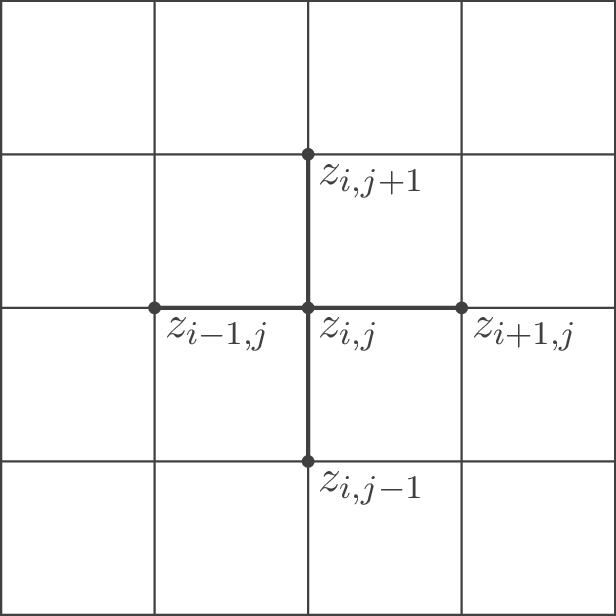
However, the wave equation also contains a second time derivative which we need to discretise as well. For the time discretisation, we simply use the physics process delta time $\Delta t$ (which is constant in Godot). We use the upper index $t$ to denote the point in time. The complete notation is $z_{i, j}^t$ for the displacement at grid coordinates $(i, j)$ and time $t$ . In order to now approximate the second time derivate, we can just use the following three-point-stencil:

$\frac{\partial^2 f(\mathbf{x}, t)}{\partial t^2} \approx \frac{z_{i, j}^{t+1} - 2 \cdot z_{i, j}^t + z_{i, j}^{t-1}}{\Delta t^2}$

Now that we have dicretized both derivatives, let’s just plug them back into the initial wave equation and solve for $z_{i, j}^{t+1}$ :

$\begin{align} 0 &= \Delta f(\mathbf{x}, t) - \frac{1}{c^2} \frac{\partial^2 f(\mathbf{x}, t)}{\partial t^2} \\ 0 &= \frac{z_{i+1, j} + z_{i, j+1} - 4 \cdot z_{i, j} + z_{i-1, j} + z_{i, j-1}}{h^2} - \frac{1}{c^2} \cdot \frac{z_{i, j}^{t+1} - 2 \cdot z_{i, j}^t + z_{i, j}^{t-1}}{\Delta t^2}\\ z_{i, j}^{t+1} &= a \cdot (z_{i+1, j}^t + z_{i, j+1}^t + z_{i-1, j}^t + z_{i, j-1}^t) + (2 - 4a) \cdot z_{i, j}^t - z_{i, j}^{t-1} \end{align}$

where we introduce $a = \frac{c^2 \Delta t^2}{h^2}$ . In order to obtain a stable simulation, $a < 0.5$ needs to hold true. We thus have some limits on our choice of $\Delta t$ and $h$, depending on how fast our waves should propagate. Grids with less points (and thus large $h$ ) are generally more stable but also less accurate. It is desirable to keep $\Delta t$ as small as reasonably possible which means high framerates will benefit our simulation.

Let’s break down the final equation: In order to update and retreive $z_{i, j}^{t+1}$ , we need to know the grid neighbouring grid values at time $t$ as well as the previous displacement values at time $t$ and $t-1$ . We can start our grid from any arbitrary initial conditions and let it evolve over time.

Now that we know the theory, let’s get to the actual implementation.

Implementation of the finite difference method

In order to bring the finite difference method to life, we use fragment shaders. Textures are basically just two-dimensional grids that can hold values (colors) at each grid point (pixel). We make use of this convenient property and simply use a texture as the grid for our finite difference method.

In the editor, we create a new viewport called SimulationViewport. This viewport in return contains a ColorRect as shown below.

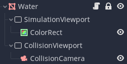
We then apply a shader to the ColorRect which contains the simulation code. The size (in pixels) of the ColorRect thus defines the size of the simulation grid. Two textures are passed as uniforms to this shader: z_tex which holds the grid values $z_{i, j}^t$ and z_old_tex which holds the grid values $z_{i, j}^{t-1}$ . The resulting values $z_{i, j}^{t+1}$ are then rendered to the ColorRect by the fragment shader. In order to retreive the current grid values, we can then simply retreive the contents of SimulationViewport with a ViewportTexture.

The snippet below contains the part of the simulation shader assigned to ColorRect which does the heavy lifting:

void fragment() {
    float pix_size = 1.0f/grid_points;

    vec4 z = a * (texture(z_tex, UV + vec2(pix_size, 0.0f))
                  + texture(z_tex, UV - vec2(pix_size, 0.0f))
		  + texture(z_tex, UV + vec2(0.0f, pix_size)) 
		  + texture(z_tex, UV - vec2(0.0f, pix_size)))
	     + (2.0f - 4.0f * a) * (texture(z_tex, UV))
	     - (texture(old_z_tex, UV));

    float z_new_pos = z.r; // positive waves are stored in the red channel
    float z_new_neg = z.g; // negative waves are stored in the green channel

    ...

    COLOR.r = z_new_pos;
    COLOR.g = z_new_neg;
}

Note that we store “positive” waves in the red and “negative” waves in the green channel. This is not particularly important now and we will explain it later on.

You can see that we first read the neighbouring grid values as well as the current and last values at the grid position and then combine them according to our formula. The resulting value is then assigned to COLOR.

a can be se at initialisation of the scene as a uniform since the physics frame rate is constant.

We also need a script that updates the simulation as well as grid textures each step. This is done in a script assigned to the Water Node. _update is called each physics frame:

func _update():
    ...
    update_height_map()

    # Render one frame of the simulation viewport to update the simulation
    simulation_viewport.render_target_update_mode = Viewport.UPDATE_ONCE

    # Wait until the frame is rendered
    yield(get_tree(), "idle_frame")
    ...

func update_height_map():
    # Update the height maps
    var img = simulation_texture.get_data() # Get currently rendered map
    # Set current map as old map
    var old_height_map = simulation_material.get_shader_param("z_tex")
    simulation_material.get_shader_param("old_z_tex") \
        .set_data(old_height_map.get_data())
    # Set the current height map from current render
    simulation_material.get_shader_param("z_tex").set_data(img)

And that’s it for our basic simulation. We now know how to propagate waves along the surface but have yet to create them.

Creating waves

When considering a boat moving through water, we need to be aware of two “types” of waves, bow waves and stern waves. Bow waves are created were the the boat’s hull pushes away the water. Stern waves, on the other hand, are created behind the boat, where water is rushing back to fill the space the boat previously occupied. We thus create positive bow waves in front of the boat and negative stern waves behind the boat. Creating positive or negative waves just means manually setting grid points to positive or negative values.

The intensity of both creatd wave types will also depend on the speed of the boat: The faster the boat, the higher the waves.

In order to create waves we first need to know where to create them. We thus need to know the intersection of the boat’s hull with the water surface.

We use a little trick to accomplish this:

Let’s create a second viewport called CollisionViewport. This viewport will hold the texture which contains the intersection areas of all objects with the surface.

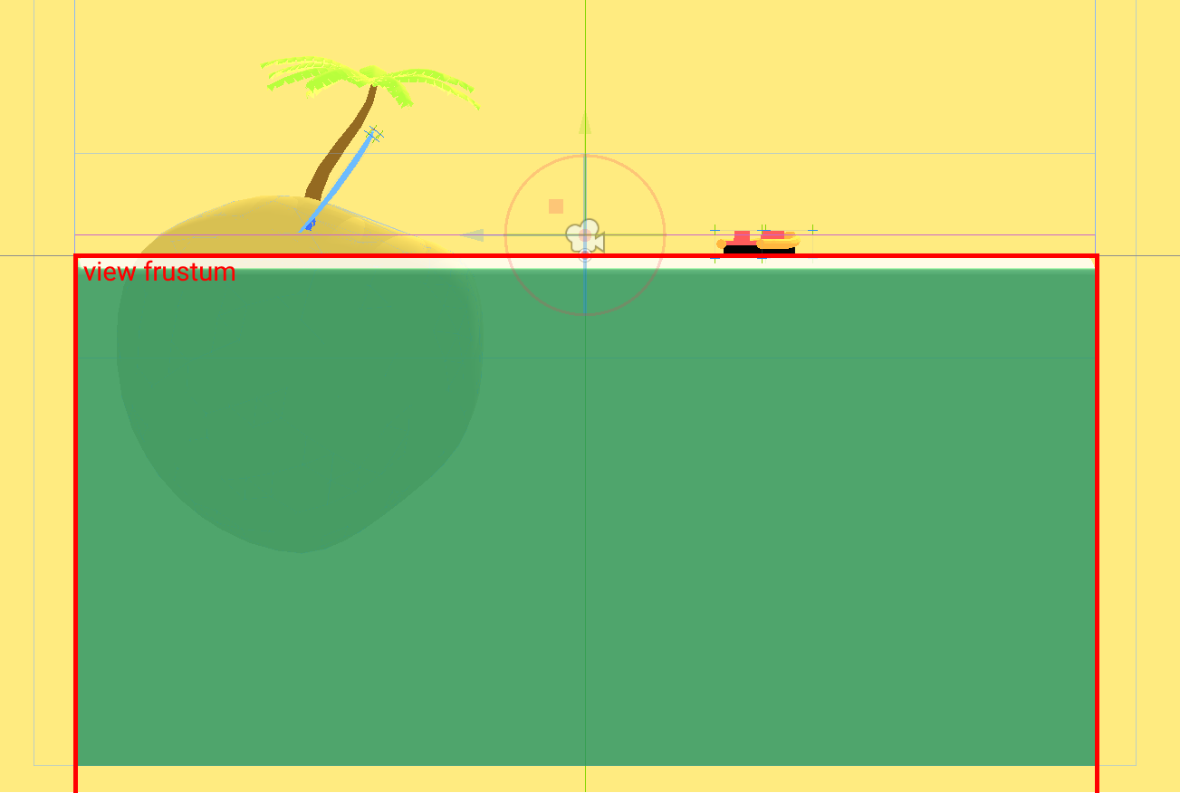
We then add a new camera called CollisionCamera to CollisionViewport. This camera uses on orthogonal projection and has its size set to that of the water surface. The near plane is set to match the water surface and the far plane should be moved sufficiently far away, as shown below.

Next, we add an additional mesh to every node that should be able to create waves and call it CollisionMesh. This mesh defines the hull of our boat.

This mesh has a special material which consists of two passes: The first one is a ShaderMaterial with a shader collision.shader that looks like this (this can also be done with a SpatialMaterial but I find this variant to be more verbose):

shader_type spatial;

uniform float speed;

render_mode cull_front;

void fragment() {
    ALBEDO.r = speed;
}

The second pass is just a SpatialMaterial with albedo set to black and a higher render priority (so that front faces are drawn in front of back faces).

The resulting material will draw the inside of the mesh whatever color we set from speed and the outside plain black. Since the camera culls every fragment above the water surface (its near plane), it will draw the colored inside of objects that intersect the surface. The viewport texture will then be black where there is no intersection and colored for all areas where a hull intersects.

We can also give information about the speed of objects to the CollisionViewport by setting the speed uniform of the shader which will then be written to the red channel.

Now that we have a texture containing the intersection of the boat hull with the surface we can pass this texture to our simulation shader and call it collision_texture. We also supply the collision texture from the last frame and call it collision_texture_old. We then read the red channels of both textures to collision_state_new and collision_state_old. By comparing these two values, we can differentiate between two important cases:

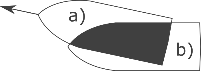
In the figure above, we create positive bow waves in area a) and negative stern waves in area b).

We add the following code to the simulation fragment shader:

void fragment() {
    ...
    float collision_state_old = texture(old_collision_texture, UV).r;
    float collision_state_new = texture(collision_texture, UV).r;

    if (collision_state_new > 0.0f && collision_state_old == 0.0f) {
        z_new_pos = amplitude * collision_state_new;
    } else if (collision_state_new == 0.0f && collision_state_old > 0.0f) {
        z_new_neg = amplitude * collision_state_old;
    }
    ...
}

As noted previously, positive waves are created on the red channel and negative waves are created on the green channel. This is perfectly fine since waves do not interact with each other and can be computed in components which are added up later (you may now this phenomenon from wave interference). The actual displacement or wave height can then be retreived by subtracting the green channel from the red channel.

We also create a function update_collision_texture in the script of the Water node which works much like update_height_map in order to set old_collision_texture and collision_texture each frame.

Below is a visualization of the collision texture on the right and the resulting displacement map on the left. You can also watch this visualisation live by making the nodes CollisionVisualisation and SimulationVisualisation visible when runnning the scene from the editor.

Land masses

Other than boats or similar moving objects we can also have land masses like islands interrupting the water surface. These objects obviously don’t move but it would still be nice to have them interact with the water by breaking waves, especially since they are often large.

This can be accomplished by passing a third type of texture to the simulation shader. We call it land_texture. Since the land masses do not move, this texture can be baked before running the scene (or crudely drawn in Paint, in my case). The land texture used for the demo scene above, for example, simply looks like this:

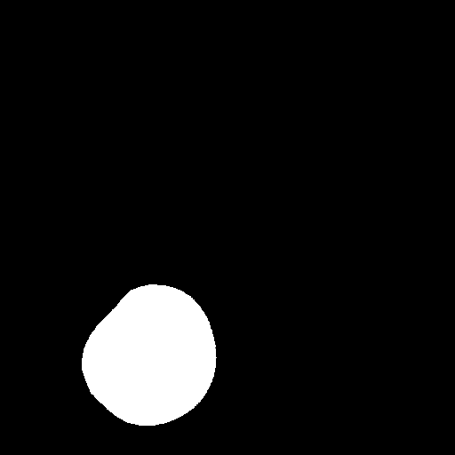
The white pixels correspond to land. We can then add a few lines to our simulation shader to prevent waves from passing through the white areas:

float land = texture(land_texture, UV).r;
if (land > 0.0f) {
    z_new_pos = 0.0f;
    z_new_neg = 0.0f;
}

Our complete simulation shader simulation.shader now looks like this:

shader_type canvas_item;

uniform float a;
uniform float amplitude;
uniform float grid_points;

uniform sampler2D z_tex;
uniform sampler2D old_z_tex;

uniform sampler2D collision_texture;
uniform sampler2D old_collision_texture;

uniform sampler2D land_texture;

void fragment() {
    float pix_size = 1.0f/grid_points;

    vec4 z = a * (texture(z_tex, UV + vec2(pix_size, 0.0f))
	          + texture(z_tex, UV - vec2(pix_size, 0.0f))
	          + texture(z_tex, UV + vec2(0.0f, pix_size)) 
	          + texture(z_tex, UV - vec2(0.0f, pix_size)))
	     + (2.0f - 4.0f * a) * (texture(z_tex, UV))
	     - (texture(old_z_tex, UV));

    float z_new_pos = z.r; // positive waves are stored in the red channel
    float z_new_neg = z.g; // negative waves are stored in the green channel

    float collision_state_old = texture(old_collision_texture, UV).r;
    float collision_state_new = texture(collision_texture, UV).r;

    if (collision_state_new > 0.0f && collision_state_old == 0.0f) {
        z_new_pos = amplitude * collision_state_new;
    } else if (collision_state_new == 0.0f && collision_state_old > 0.0f) {
        z_new_neg = amplitude * collision_state_old;
    }

    float land = texture(land_texture, UV).r;
    if (land > 0.0f) {
        z_new_pos = 0.0f;
        z_new_neg = 0.0f;
    }

    COLOR.r = z_new_pos;
    COLOR.g = z_new_neg;
}

We have to implement one last step to make our simulation complete.

Buoyant RigidBodys

We can create waves now but in case we want to create an actual boat as a RigidBody, it will still simply fall through the water never to be seen again. In order to prevent this, we need to implement some form of buoyancy.

For this, we create a new node, called BuoyancyProbe. The script of this node is quite short:

extends Spatial

export var buoyancy = 5.0
export var drag = 0.18 # Drag factor (total dampening is buoyancy*drag)

var water_node : Node

var force : float = 0.0

var velocity = Vector3(0.0, 0.0, 0.0)
var old_pos = Vector3(0.0, 0.0, 0.0)

func _physics_process(delta):
    if water_node:
        # Approximate the current velocity (needed for drag)
        var pos = global_transform.origin
        velocity = (pos - old_pos) / delta
        old_pos = pos

        # Get height of water at current position and calculate
        # the current displacement.
        var h = water_node.get_height(global_transform.origin)
        var disp = global_transform.origin.y - h
        if (disp < 0):
            force = buoyancy*(-disp - drag * velocity.y)
        else:
            # No force if above water
            force = 0.0

The BuoyancyProve detects how far it is currently submerged by retreiving the current height of the water surface via the function get_height on the Water node which is defined there as follows:

func _physics_process(delta):
    _update()
    surface_data = simulation_texture.get_data().get_data()
	
func get_height(global_pos):
    # Get the height at the 
    var local_pos = to_local(global_pos)

    # Get pixel position
    var y = int((local_pos.x + water_size / 2.0) / water_size * (grid_points))
    var x = int((local_pos.z + water_size / 2.0) / water_size * (grid_points))

    # Just return a very low height when not inside texture
    if x > grid_points - 1 or y > grid_points - 1 or x < 0 or y < 0:
        return -99999.9

    # Get height from surface data (in RGB8 format)
    # This is faster than locking the image and using get_pixel()
    var height = mesh_amplitude * (surface_data[3*(x*(grid_points) + y)] \
    				 - surface_data[3*(x*(grid_points) + y) + 1]) \
				/ 255.0
    return height

We read directly from the raw data of the SimulationViewport’s texture so that we don’t have to lock the image for a pixel read for every BuoyancyProbe in the scene which would get very slow.

In case the BuoyancyProbe detects that it is underwater, it sets its force property to a value that depends linearly on the submergence depth (minus some drag). Note, that this is not physically correct as the buoyant force would actually depend on the mass that has been displaced by the body. Archimides does actually look a bit sad:

However, a linear force will nicely go to zero at the water surface which makes for a much smoother simulation.

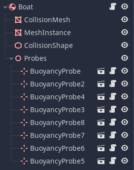
We can now add BuoyancyProbes at strategic positions to RigidBodys that we want to be buoyant and accumulate the resulting forces from a script like this (all probes are children of a child Spatial node that is called probes in the script):

for i in range(probes.get_child_count()):
    if probes.get_child(i).force > 0.0:
        add_force(Vector3(0.0, \
			  probes.get_child(i).force, \
			  0.0) / probes.get_child_count(), \
		  probes.get_child(i).global_transform.origin \
		  - global_transform.origin)

Here is the hierarchy in the editor:

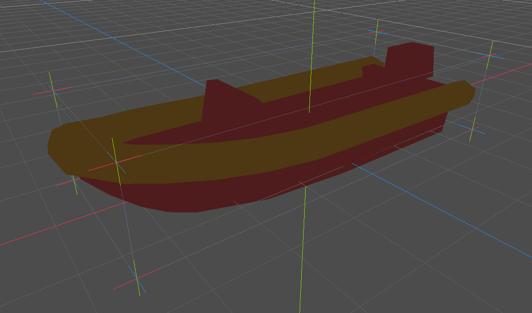
And this are the probe positions of the boat:

And that’s it! Our simulation is complete! We still need to visualize the water surface though by reading from the SimulationViewport.

Graphics

Visualising the water surface is quite easy. We already have the displacement/height map stored in the red and green channels of the SimulationViewport’s texture. The idea is to read these values and set the vertex positions and normals of the water surface inside a shader accordingly.

For this, we create a simple cuboid in Blender. Round the edges a bit to make it more visually pleasing and then subdivide the top face of the cuboid into a grid. Note that this grid does not need to have the same resolution as the simulation grid as we will add detail in the fragment shader. For me, 200 x 200 vertices achieved reasonably pleasing results. Then let us set the vertex colors of the grid vertices (that is the vertices that should actually be displaced) to red while leaving all the other vertices black and mapped the surface so that the UVs on the grid go from 0 to 1 in both directions.

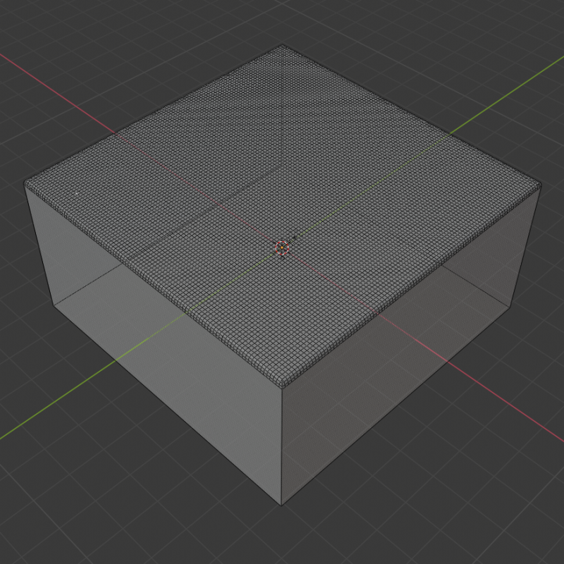
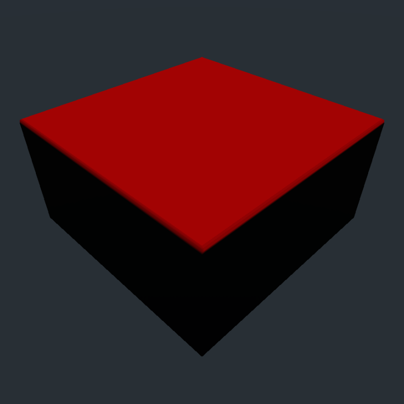
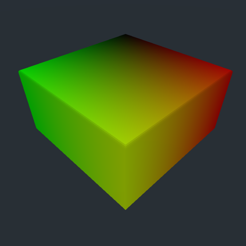
I exported the mesh using the Godot Engine Exporter for Blender since we need support for vertex colors.

Back in Godot, we then simply add a shader to the mesh and displace the vertices by reading from the height map:

void vertex() {
    if (COLOR.r > 0.0f && texture(collision_texture, UV).r == 0.0f) {
	vec4 tex = texture(simulation_texture, UV);
	float height = tex.r - tex.g;
	VERTEX.y += amplitude * COLOR.r * height;
    }
}

We also multiply the resulting height with the vertex color to make the transition a bit smoother towards the edges.

We add detail by also calculating the normals in the fragment shader:

void fragment() {
    if (COLOR.r > 0.0f) {
	float v = COLOR.r;
	vec4 tex = texture(simulation_texture, UV);
	vec4 tex_dx = texture(simulation_texture, UV + vec2(0.01, 0.0));
	vec4 tex_dy = texture(simulation_texture, UV + vec2(0.0, 0.01));
	float height = tex.r - tex.g;
	float height_dx = tex_dx.r - tex_dx.g;
	float height_dy = tex_dy.r - tex_dy.g;
	NORMAL = COLOR.r
		 * normalize(mat3(INV_CAMERA_MATRIX)
		   	     * (vec3(height_dx - height,
			             1.0,
				     height_dx - height)
				/ 0.01))
		 + (1.0f - COLOR.R) * NORMAL;
    }	
    ...
}

Note, that in the first line of the vertex shader

if (COLOR.r > 0.0f && texture(collision_texture, UV).r == 0.0f) ...

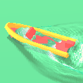
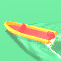
we do not only check the vertex color but also the collision texture from CollisionViewport. This is to prevent waves from “glitching” through the boat: We do not visualise waves when the boat is currently passing through them. Below is a comparison without and with this tweak in place:

Conclusion

I hope this tutorial was somewhat helpful to you. If you’d like, you can leave feedback over at my Twitter @CaptainProton42 or directly on GitHub.

There are still many possibilities to expand this method: Using multiple grids for infinite water surfaces, choosing a more stable integration scheme or more advanced hull modelling. I repeat my advice to read Real-Time Open Water Environments with Interacting Objects by H. Cords and O. Staadt for ideas on approaches.